If the workbook was open for at least 10 minutes and created an AutoRecover version, Excel kept a copy for you.
Follow these steps to get it back:
- Open Excel.
- In the left panel, choose Open Other Workbooks.
In the center panel, scroll all the way to the bottom of the recent files. At the very end, click Recover Unsaved Workbooks.

Excel shows you all the unsaved workbooks that it has saved for you recently.

- Click a workbook and choose Open. If it is the wrong one, go back to File, Open and scroll to the bottom of the list.
When you find the right file, click the Save As button to save the workbook. Unsaved workbooks are saved for four days before they are automatically deleted.

Use AutoRecover Versions to Recover Files Previously Saved
Recover Unsaved Workbooks applies only to files that have never been saved. If your file has been saved, you can use AutoRecover versions to get the file back. If you close a previously saved workbook without saving recent changes, one single AutoRecover version is kept until your next editing session. To access it, reopen the workbook. Use File, Info, Versions to open the last AutoRecover version.
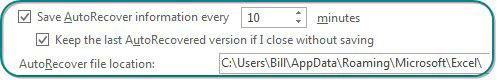
You can also use Windows Explorer to search for the last AutoRecover version. The Excel Options dialog box specifies an AutoRecover File Location. If your file was named Budget2020Data, look for a folder within the AutoRecover File folder that starts with Budget.
While you are editing a workbook, you can access up to the last five AutoRecover versions of a previously saved workbook. You can open them from the Versions section of the Info category. You may make changes to a workbook and want to reference what you previously had. Instead of trying to undo a bunch of revisions or using Save As to save as a new file, you can open an AutoRecover version. AutoRecover versions open in another window so you can reference, copy/paste, save the workbook as a separate file, etc.
Note
An AutoRecover version is created according to the AutoRecover interval AND only if there are changes. So if you leave a workbook open for two hours without making any changes, the last AutoSave version will contain the last revision.
Caution
Both the Save AutoRecover Information option and Keep The Last AutoRecovered Version option must be selected in File, Options, Save for this to work.
Tip
Create a folder called C:\AutoRecover\ and specify it as the AutoRecover File Location. It is much easier than trawling through the Users folder that is the default location.
Note
Under the Manage Version options on the Info tab you can select Delete All Unsaved Workbooks. This is an important option to know about if you work on public computers. Note that this option appears only if you’re working on a file that has not been saved previously. The easiest way to access it is to create a new workbook.
Comments
Post a Comment