
Create Sum that gives summary of all Worksheets in Excel

 You have a workbook with 12 worksheets, 1 for each month. All of the worksheets have the same number of rows and columns. You want a summary worksheet in order to total January through December.

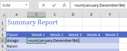
To create it, use the formula =SUM(January:December!B4).

After sheets for January through December, a new Summary worksheet is shown. The formula =SUM(January:December!B4) is in B4.

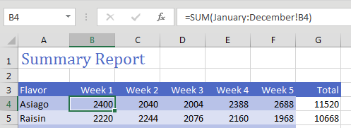
Copy the formula to all cells and you will have a summary of the other 12 worksheets.

Copy the formula throughout the worksheet and you will have a report adding up the similar cell on the 12 monthly worksheets.

Caution

I make sure to never put spaces in my worksheet names. If you do use spaces, the formula would have to include apostrophes, like this: =SUM('Jan 2018:Mar 2018'!B4).

Comments

Popular posts from this blog

DAX Language - Data Analysis Expression

The DAX language was created specifically for the handling of data models, through the use of formulas and expressions. DAX is used in several Microsoft Products such as Microsoft Power BI, Microsoft Analysis Services and Microsoft Power Pivot for Excel. Below are the types of Dax functions  1. Aggregate  2. Date and time 3. Filter 4. Financial  5. Information  6. Logical 7. Maty and trig 8. Other 9. Parent and child 10. Relationship Management  11. Statistical  12. Table manipulation  13. Text 14. Time intelligence  From the above list of functions 3 types of functions are basic and commonly used, those are Aggregate , Logical and Date and time. Other important entities which are used with the above function are as follows  1. Operators  Example -  ( ), + , Not, &, =, < >, || 2. Statements  Define , Evaluate,  Order by, Return, Var 3. Data Types Binary, boolean,  Currency,  date time, decimal, integer,...

CAGR Dax Measure

CAGR stands for  C ompound  A nnual  G rowth  R ate.  It describes the rate at which an investment would have grown over several years if it had grown at the same rate every year on a compounding, rather than simple, basis.   The CAGR metric is calculated using the following formula: If we were to fit this entire formula into a single measure it may get messy and confusing for other users, so let’s step it out. We will need to create several measures to calculate the individual pieces the CAGR formula.  Of course, this is not the only way to calculate CAGR in Power Pivot, but this is the way we’ve decided to go about it.  So, let’s break it down, we will need the following measures to calculate CAGR: A measure to retrieve the First Year in the data set A measure to retrieve the Last Year in the data set A measure to calculate the Number of Years between the First and Last Years in the data set A measure to aggregate the total sales in the data set...

40 Power Query Editor features in Power BI

40 Power Query Editor features in Power BI along with examples: 1. Filter Rows: Remove rows based on conditions. Example: Remove rows with a null value in the "CustomerName" column. 2. Remove Duplicates: Eliminate duplicate rows. Example: Remove duplicate entries based on the "OrderID" column. 3. Sort Rows: Arrange rows in ascending or descending order. Example: Sort data by "Date" column in descending order. 4. Replace Values: Substitute one value with another. Example: Replace "N/A" with "Unknown" in the "Status" column. 5. Split Columns: Divide a column into multiple columns. Example: Split "FullName" into "FirstName" and "LastName." 6. Merge Queries: Combine data from multiple sources. Example: Merge customer and order data based on the "CustomerID." 7. Group By: Aggregate data based on a specific column. Example: Group sales data by "ProductCategory" and calculate the sum ...