
Power Query - Excel's most powerful tool


Power Query cleans and transforms data

Power Query Process Overview Steps - Transform Data
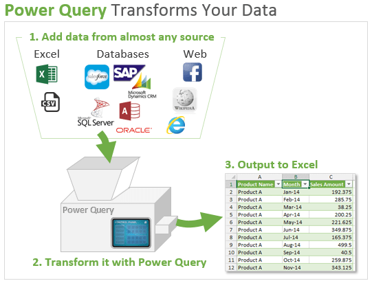
  1. You add your data sources (Excel tables, CSV files, database tables, webpages, etc.)
  2. Press buttons in the Power Query Editor window to transform your data.
  3. Output that data to your worksheet or data model (PowerPivot) that is ready for pivot tables or reporting.

Power Query is like a machine because once you have your query setup, the process can be repeated with the click of a button (refresh) every time your data changes.

If you have used macros to transform your data, you can think of this as a much easier alternative to VBA that does NOT require coding.

Common Data Tasks Made Easy

Do you work with data that has been exported from a system of record?  This could be a general ledger, accounting, ERP, CRM, Salesforce.com, or any reporting system that contains data.

If so, you probably spend a lot of time transforming or re-shaping your data to create additional reports, pivot tables, or charts.

Unpivot Exported Data with Power Query in Excel

These data transformations could include tasks like:

  • Remove columns, rows, blanks
  • Convert data types – text, numbers, dates
  • Split or merge columns
  • Sort & filter columns
  • Add calculated columns
  • Aggregate or summarize data
  • Find & replace text
  • Unpivot data to use for pivot tables

Do any of these tasks sound familiar?  If so, then they probably also sound boring, repetitive, and time consuming. 🙂  Believe me, I’ve spent the better part of my career doing these tasks and trying to figure out faster ways to get them done.

Fortunately, Power Query has buttons that automate all these tasks!

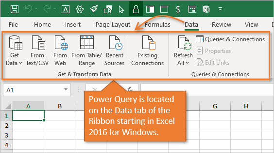
Overview of the Power Query Ribbon

Starting in Excel 2016 for Windows, Power Query has been fully integrated into Excel.  It is now on the Data tab of the Ribbon in the Get & Transform group.

Power Query Get and Transform Data Tab of Ribbon Excel 2016 2019 Office 365 Microsoft 365

In Excel 2010 and 2013 for Windows, Power Query is a free add-in.  Once installed, the Power Query tab will be visible in the Excel Ribbon.

Power Query Ribbon for Excel v2.16.3785.242
Click to Enlarge

You use the buttons in the Data or Power Query tab to get your source data.  Again, your data could be stored in Excel files, csv files, Access, SQL server database, SharePoint, Salesforce.com, Dynamics CRM, Facebook, Wikipedia, websites, and more.

Once you have specified where your data is coming from, you then use the Power Query Editor window to make transformations to the data.

Power Query Editor Window Home Tab Transform Data with Buttons

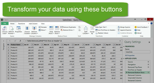
The buttons in the Power Query Editor Window allow you to transform your data.

Power Query Editor Window Home and Transform Tab Buttons

Think about some of those tasks you do repeatedly as you browse the buttons in the image above.  Each time you press a button your actions (steps) are recorded, and you can quickly re-apply the steps when you receive new data by refreshing the query.

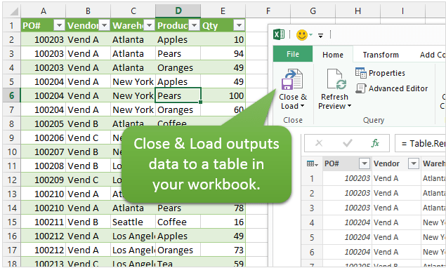
After completing your steps, you can output the data to a Table in your Excel workbook by clicking the Close & Load button.

Close and Load Button in Power Query Editor Window

You can also modify existing queries and refresh your output tables with the changes or updated data.

Data Transformation Examples

Here are a few examples of what Power Query can do with your data.

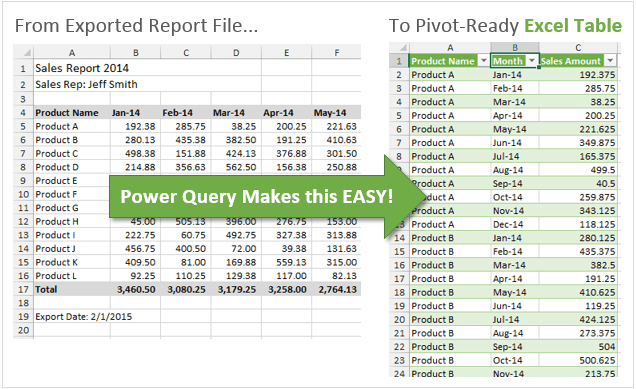
Unpivot Data for Pivot Tables

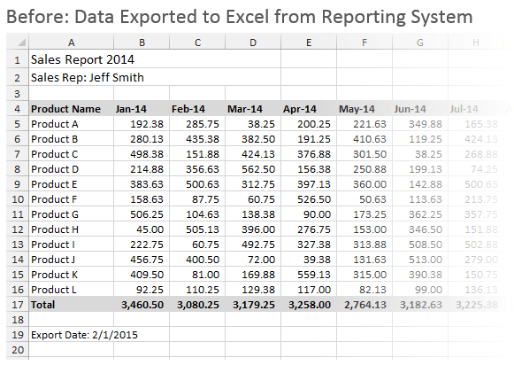
My favorite feature of Power Query is it’s ability to Unpivot data.  This is a technique used to get your data ready for the source of a pivot table.  This is also referred to as normalizing your data to get it in a tabular format.

The data might start out looking something like the following.

Exported Report Data in ExcelFile

And you want the end result to look like this.

Unpivot Data with Power Query for use in Pivot Table

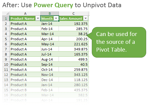
Power Query can do this with the click of a few buttons, and prepare your data for use in a pivot table.

Comments

Popular posts from this blog

Data Cleaning Functions in Excel

  The CLEAN function Using the CLEAN function removes nonprintable characters text. For example, if the text labels shown in a column are using crazy nonprintable characters that end up showing as solid blocks or goofy symbols, you can use the CLEAN function to clean up this text. The cleaned‐up text can be stored in another column. You can then work with the cleaned text column. The CLEAN function uses the following syntax: CLEAN(text) The text argument is the text string or a reference to the cell holding the text string that you want to clean. For example, to clean the text stored in Cell A1, use the following syntax: CLEAN(A1) The CONCATENATE function The CONCATENATE function combines, or joins, chunks of text into a single text string. The CONCATENATE function uses the following syntax: CONCATENATE(text1,text2,text3,...) The text1, text2, text3, and so on arguments are the chunks of text that you want to combine into a single string. For example, if the city, state, and ZIP co...

Formatting Tips

1. Use tables to format data quickly Excel Tables  are an incredibly powerful way to handle a bunch of related data. Just select any cell with in the data and press CTRL+T and then Enter. And bingo, your data looks slick in no time. This has to be the best and easiest formatting tip. 2. Change colors in a snap So you have made a spreadsheet model or dashboard. And you want to change colors to something fresh. Just go to Page Layout ribbon and choose a color scheme from Colors box on top left. Microsoft has defined some great color schemes. These are well contrasted and look great on your screen. You can also define your own color schemes (to match corporate style). What more, you can even define schemes for fonts or combine both and create a new theme. 3. Use cell styles Consistency is an important aspect of formatting. By using cell styles, you can ensure that all similar information in your workbook is formatted in the same way. For example, you can color all input cells in orang...

Rank Function

How to Use the RANK Function If you give the RANK function a number, and a list of numbers, it will tell you the rank of that number in the list, either in ascending or descending order. For example, in the screen shot below, there is a list of 10 student test scores, in cells B2:B11. To find the rank of the the first student's score in cell B2, enter this formula in cell C2: =RANK(B2,$B$2:$B$11) Then, copy the formula from cell C2 down to cell C11, and the scores will be ranked in descending order. RANK Function Arguments There are 3 arguments for the RANK function: number : in the above example, the number to rank is in cell  B2 ref : We want to compare the number to the list of numbers in cells  $B$2:$B$11 . Use an absolute reference ($B$2:$B11), instead of a relative reference (B2:B11)so the referenced range will stay the same when you copy the formula down to the cells below order : (optional) This argument tells Excel whether to rank the list in ascending or descending o...