Protect Formula Cells in Excel

The use of worksheet protection in Excel is a little strange. Using the steps below, you can quickly protect just the formula cells in your worksheet.

It seems unusual, but all 16 billion cells on a worksheet start out with their Locked property set to True. You need to unlock all of the cells first:

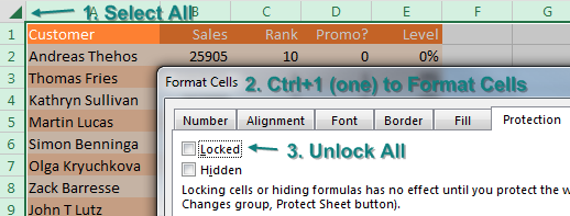
Select all cells by using the icon above and to the left of cell A1.
Press Ctrl+1 (that is the number 1) to open the Format Cells dialog.
In the Format Cells dialog, go to the Protection tab. Uncheck Locked. Click OK.

Select all cells and change the Locked property to off.

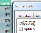
While all cells are still selected, select Home, Find & Select, Formulas.

At this point, only the formula cells are selected. Press Ctrl+1 again to display the Format Cells dialog. On the Protection tab, choose Locked to lock all of the formula cells.

With only the formula cells selected, set Locked property to On.

Locking cells does nothing until you protect the worksheet. On the Review tab, choose Protect Sheet. In the Protect Sheet dialog, choose if you want people to be able to select your formula cells or not.

Comments

Change from Lower to Upper Case in Excel

1. Insert a new blank column to the right of your data. 2. Use a formula such as =UPPER(D2) . To convert to lower case, use =LOWER() . To convert to Proper case, use =PROPER() . 3. Copy the temporary formula down to all rows by double-clicking the fill handle. 4. The entire range of new formulas will be selected. Press Ctrl+C to copy. 5. Press the left arrow to move to the original data. Right-click and choose Paste Values. 6. You can now delete the temporary column D. Additional Details : I to bring up the “W” program again, but here is another place where Microsoft Word could make this easier. If you had an entire table that needs converting, select the whole table, paste to a blank word document, then use the Change Case dropdown in the Home tab. After the conversion is done, copy from Word and paste back to Excel. #upper #Uppercase

Recover Unsaved Excel File

We normally avoid these settings but in the hour of need they save us rework time. So if your working on a excel file and you forget to save it or click on don't save by mistake, follow below steps If the workbook was open for at least 10 minutes and created an AutoRecover version, Excel kept a copy for you. Follow these steps to get it back: Open Excel. In the left panel, choose Open Other Workbooks. In the center panel, scroll all the way to the bottom of the recent files. At the very end, click Recover Unsaved Workbooks. Excel shows you all the unsaved workbooks that it has saved for you recently. Click a workbook and choose Open. If it is the wrong one, go back to File, Open and scroll to the bottom of the list. When you find the right file, click the Save As button to save the workbook. Unsaved workbooks are saved for four days before they are automatically deleted. Use AutoRecover Versions to Recover Files Previously Saved Recover Unsaved Workbooks applies only to files that...

How many types of the predefined freeze panes are there in Excel?

Freeze Panes in Excel is used to fix any frame or row or section of the table to access the data located so down below so that the user can see the header’s name as well. There is 3 type of Freeze Panes option available in View menu tab under Window section, Freeze Panes, Freeze Top Row and Freeze First Column. Freeze Panes is used to freeze the worksheet from the point where we keep our cursor. This freezes both the row and column both. Then to freeze a Row and a Column, we have a separate option to freeze each of them. Once we do that, we will see some portion of the worksheet will not move until we unfreeze it.

Solutions for Data Science

Search This Blog