Indirect Function

INDIRECT is pretty cool for grabbing a value from a cell. Can INDIRECT point to a multi-cell range and be used in a VLOOKUP or SUMIF function?

You can build an INDIRECT function that points to a range. The range might be used as the lookup table in a VLOOKUP or as a range in SUMIF or COUNTIF.

In Figure, the formula pulls data from the worksheets specified in row 4. The second argument in the SUMIF function looks for records that match a certain date from column A.

Note: Because each worksheet might have a different number of records, I chose to have each range extend to 300. This is a number that is sufficiently larger than the number of transactions on any sheet. The formula in cell B5 is:

=SUMIF(INDIRECT(B$4&"!A2:A300"), $A5, INDIRECT(B$4&"!C2:C300"))

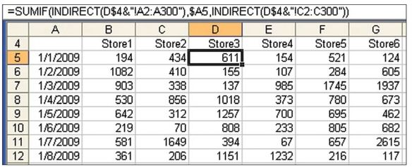
Figure 36. Each INDIRECT points to a rectangular range on the other worksheet.

Summary: You can use INDIRECT to grab data from a multi-cell range.

Comments

Rank Function

How to Use the RANK Function If you give the RANK function a number, and a list of numbers, it will tell you the rank of that number in the list, either in ascending or descending order. For example, in the screen shot below, there is a list of 10 student test scores, in cells B2:B11. To find the rank of the the first student's score in cell B2, enter this formula in cell C2: =RANK(B2,$B$2:$B$11) Then, copy the formula from cell C2 down to cell C11, and the scores will be ranked in descending order. RANK Function Arguments There are 3 arguments for the RANK function: number : in the above example, the number to rank is in cell B2 ref : We want to compare the number to the list of numbers in cells $B$2:$B$11 . Use an absolute reference ($B$2:$B11), instead of a relative reference (B2:B11)so the referenced range will stay the same when you copy the formula down to the cells below order : (optional) This argument tells Excel whether to rank the list in ascending or descending o...

Compare two columns with Go To Special

In the figure below, say that you want to find any changes between column A and column D. Select the data in A2:A9 and then hold down the Ctrl key while you select the data in D2:D9. Select, Home, Find & Select, Go To Special. Then, in the Go To Special dialog, choose Row Differences. Click OK. Only the items in column A that do not match the items in column D are selected. Use a red font to mark these items, as shown below. Caution This technique works only for lists that are mostly identical. If you insert one new row near the top of the second list, causing all future rows to be offset by one row, each of those rows is marked as a row difference

Vlookup to the Left with Index and Match function

What if your lookup value is to the right of the information that you want VLOOKUP to return? Conventional wisdom says VLOOKUP cannot handle a negative column number in order to go left of the key. One solution is =VLOOKUP(I7,CHOOSE({1,2},G1:G5,F1:F5),2,0) . However, I prefer to use MATCH to find where the name is located and then use INDEX to return the correct value.

Solutions for Data Science

Search This Blog