
Power Query Basics - Clean Raw Data and reuse the file for updating new data

Download Example File from link below
https://drive.google.com/file/d/1FnYGYGfTnFEeMwI-EZS89xgIOklrNBNA/view?usp=sharing


Power Query is built in to Windows versions of Office 365, Excel 2016, Excel 2019 and is available as a free download in Windows versions of Excel 2010 and Excel 2013. The tool is designed to extract, transform, and load data into Excel from a variety of sources. The best part: Power Query remembers your steps and will play them back when you want to refresh the data. This means you can clean data in 80% of the normal time

I say this about a lot of new Excel features, but this really is the best feature to hit Excel in 20 years.

Get Power Query

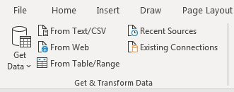
You may already have Power Query. It is in the Get & Transform group on the Data tab.

The Get & Transform Data group includes Get Data, From Text/CSV, From Web, From Table/Range, Recent Sources, Existing Connections.

But if you are in Excel 2010 or Excel 2013, go to the Internet and search for Download Power Query. Your Power Query commands will appear on a dedicated Power Query tab in the Ribbon.

Clean Data the First Time in Power Query

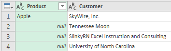
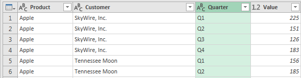
To give you an example of some of the awesomeness of Power Query, say that you get the file shown below every day. Column A is not filled in. Quarters are going across instead of down the page.

To start, save that workbook to your hard drive. Put it in a predictable place with a name that you will use for that file every day.


In Excel, select From Table under Data tab.


Power Query Window will appear.


Now you need to fix all the blank cells in column A. If you were to do this in the Excel user interface, the unwieldy command sequence is Home, Find & Select, Go To Special, Blanks, Equals, Up Arrow, Ctrl+Enter.

The blank cells in column A now say "null" in the Power Query Editor.

In Power Query, select Transform, Fill, Down.

Choose column A. Open the Fill drop-down menu and choose FIll, Down.

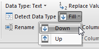
All of the null values are replaced with the value from above. With Power Query, it takes three clicks instead of seven.

Next problem: The quarters are going across instead of down. In Excel, you can fix this with a Multiple Consolidation Range pivot table. This requires 12 steps and 23+ clicks.

In Power Query select the two columns that are not quarters. Open the Unpivot Columns dropdown on the Transform tab and choose Unpivot Other Columns, as shown below.

Select columns A and B in Power Query. On the Ribbon, choose Unpivot other columns.

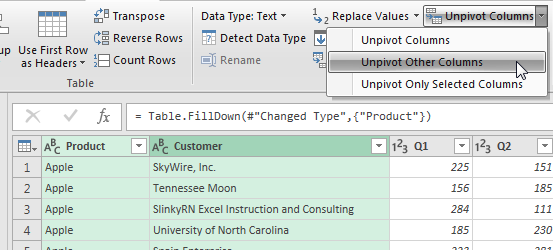
Right-click on the newly created Attribute column and rename it Quarter instead of Attribute. Twenty-plus clicks in Excel becomes five clicks in Power Query.

You have four times as many rows. Columns A & B appear the same (except there are four rows for each previous one row). The Quarters that were going across columns C, D, E, and F now go down column C. The revenue from the data set is now in column D.

Now, to be fair, not every cleaning step is shorter in Power Query than in Excel. Removing a column still means right-clicking a column and choosing Remove Column. But to be honest, the story here is not about the time savings on Day 1.

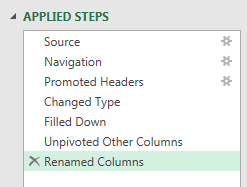
Power Query Remembers All of Your Steps

Look on the right side of the Power Query window. There is a list called Applied Steps. It is an instant audit trail of all of your steps. Click any gear icon to change your choices in that step and have the changes cascade through the future steps. Click on any step for a view of how the data looked before that step.

On the right side of the Power Query Editor, a list of Applied Steps. For this example, you have Source, Navigation, Promoted Headers, Changed Type, Filled Down, Unpivoted Other Columsn, Renamed Columns.

When you are done cleaning the data, click Close & Load To as shown below.

Tip

If your data is more than 1,048,576 rows, you can use the Close & Load dropdown to load the data directly to the Power Pivot Data Model, which can accommodate 995 million rows if you have enough memory installed on the machine.


Select New Worksheet and Table then click on load


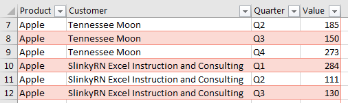
In a few seconds, your transformed data appears in Excel. Awesome.

The transformed data is returned to a table in Excel.

The Payoff: Clean Data With One Click

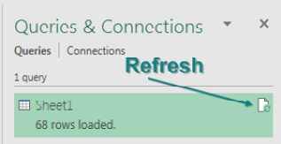
But again, the Power Query story is not about the time savings on Day 1. When you select the data returned by Power Query, a Queries & Connections panel appears on the right side of Excel, and on it is a Refresh button. (We need an Edit button here, but because there isn't one, you have to right-click the original query to view or make changes to the original query).

The Queries & Connections panel lists one query called Sheet1 with 68 rows loaded. If you make the panel wider and hover over Sheet1, a refresh icon appears.

You can add more data under the Raw data and click on Refresh. New data will be updated automatically.

Click on Show queries if the Right pane doesn't appear.


This is just a example of what power query can do. I will upload more posts for other features of Power Query.

Comments

Popular posts from this blog

DAX Language - Data Analysis Expression

The DAX language was created specifically for the handling of data models, through the use of formulas and expressions. DAX is used in several Microsoft Products such as Microsoft Power BI, Microsoft Analysis Services and Microsoft Power Pivot for Excel. Below are the types of Dax functions  1. Aggregate  2. Date and time 3. Filter 4. Financial  5. Information  6. Logical 7. Maty and trig 8. Other 9. Parent and child 10. Relationship Management  11. Statistical  12. Table manipulation  13. Text 14. Time intelligence  From the above list of functions 3 types of functions are basic and commonly used, those are Aggregate , Logical and Date and time. Other important entities which are used with the above function are as follows  1. Operators  Example -  ( ), + , Not, &, =, < >, || 2. Statements  Define , Evaluate,  Order by, Return, Var 3. Data Types Binary, boolean,  Currency,  date time, decimal, integer,...

What if Analysis

Sometimes, you want to see many different results from various combinations of inputs. Provided that you have only two input cells to change, the Data Table feature will do a sensitivity analysis. Using the loan payment example, say that you want to calculate the price for a variety of principal balances and for a variety of terms. Make sure that the formula you want to model is in the top-left corner of a range. Put various values for one variable down the left column and various values for another variable across the top. From the Data tab, select What-If Analysis, Data Table.... You have values along the top row of the input table. You want Excel to plug those values into a certain input cell. Specify that input cell for Row Input Cell. You have values along the left column. You want those plugged into another input cell. Specify that cell for the Column Input Cell. When you click OK, Excel repeats the formula in the top-left column for all combinations of the top row and left colum...

20 Time Intelligence Dax Measures

20 Time Intelligence DAX measures in Power BI with examples: Year-to-Date Sales: css Copy code YTD Sales = TOTALYTD( [Total Sales] , Calendar [Date] ) Month-to-Date Sales: css Copy code MTD Sales = TOTALMTD( [Total Sales] , Calendar [Date] ) Quarter-to-Date Sales: css Copy code QTD Sales = TOTALQTD( [Total Sales] , Calendar [Date] ) Previous Year Sales: mathematica Copy code Previous Year Sales = CALCULATE ( [ Total Sales ] , SAMEPERIODLASTYEAR ( Calendar [ Date ] ) ) Year-over-Year Growth: css Copy code YoY Growth = DIVIDE( [Total Sales] - [Previous Year Sales] , [Previous Year Sales] ) Rolling 3-Month Average Sales: sql Copy code 3 M Rolling Avg Sales = AVERAGEX(DATESINPERIOD(Calendar[ Date ], MAX (Calendar[ Date ]), -3 , MONTH ), [Total Sales]) Cumulative Sales: scss Copy code Cumulative Sales = SUMX (FILTER(ALL(Calendar), Calendar [Date] <= MAX (Calendar[Date])), [Total Sales] ) Running Total Sales: scss Copy code Running Total Sales = SUMX (FILTER(ALL(Calendar), Calen...