Protect rows from getting deleted

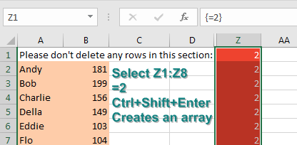
Instructions on the worksheet ask people not to delete any rows. Someone will try to delete a row. Off to the right, select Z1:Z8. Type =2 and press Ctrl+Shift+Enter. This creates an array in those rows.

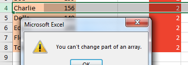
If someone tries to delete a row, Excel prevents it and shows a cryptic message about arrays, shown below.

When someone tries to delete a row in the area of rows 1 to 8, a message will appear with "You Can't Change Part Of an Array."

Comments

3D Map in Excel

3D Maps ( Power Map) is available in the Office 365 versions of Excel 2013 and all versions of Excel 2016. Using 3D Maps, you can build a pivot table on a map. You can fly through your data and animate the data over time. 3D Maps lets you see five dimensions: latitude, longitude, color, height, and time. Using it is a fascinating way to visualize large data sets. 3D Maps can work with simple one-sheet data sets or with multiple tables added to the Data Model. Select the data. On the Insert tab, choose 3D Map. (The icon is located to the right of the Charts group.) If you have Excel 2013 you might have to download Power Map Preview from Microsoft to use the feature. Next, you need to choose which fields are your geography fields. This could be Country, State, County, Zip Code, or even individual street addresses. You are given a list of the fields in your data set and drop zones named Height, Category, and Time. Hover over any point on the map to get details such as last sale date and a...

CAGR Dax Measure

CAGR stands for C ompound A nnual G rowth R ate. It describes the rate at which an investment would have grown over several years if it had grown at the same rate every year on a compounding, rather than simple, basis. The CAGR metric is calculated using the following formula: If we were to fit this entire formula into a single measure it may get messy and confusing for other users, so let’s step it out. We will need to create several measures to calculate the individual pieces the CAGR formula. Of course, this is not the only way to calculate CAGR in Power Pivot, but this is the way we’ve decided to go about it. So, let’s break it down, we will need the following measures to calculate CAGR: A measure to retrieve the First Year in the data set A measure to retrieve the Last Year in the data set A measure to calculate the Number of Years between the First and Last Years in the data set A measure to aggregate the total sales in the data set...

Turn Data Sideways

Someone built this lookup table sideways, stretching across C1:N2. I realize that I could use HLOOKUP instead of VLOOKUP, but I prefer to turn the data back to a vertical orientation. Copy C1:N2. Right-click in A4 and choose the Transpose option under the Paste Options. Transpose is the fancy Excel word for “turn the data sideways.” I transpose a lot. But I use Alt+E , S , E , Enter to transpose instead of the right-click. There is a problem, though. Transpose is a one-time snapshot of the data. What if you have formulas in the horizontal data? Is there a way to transpose with a formula? The first way is a bit bizarre. If you are trying to transpose 12 horizontal cells, you need to select 12 vertical cells in a single selection. Start typing a formula such as =TRANSPOSE(C2:N2) in the active cell but do not press Enter. Instead, hold down Ctrl+Shift and then press Enter . This puts a single array formula in the selected cells. T...

Solutions for Data Science

Search This Blog