Goal Seek feature in Excel


Have you ever found yourself plugging in successively higher and lower values into an input cell, hoping to arrive at a certain answer?


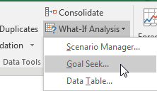
A tool that is built in to Excel does exactly this set of steps. Select the cell with the Payment formula. On the Data tab, in the Data Tools group, look for the What-If Analysis dropdown and choose Goal Seek….
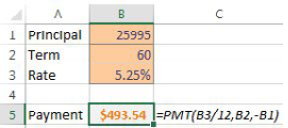
A simple model calculates a loan payment. Choose the payment cell.
Under What-If Analysis, choose Goal Seek.

The figure below shows how you can try to set the payment in B5 to $425 by changing cell B1
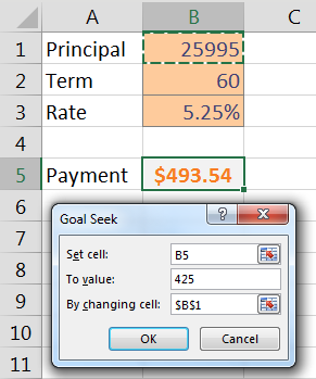
In the Goal Seek dialog, Set Cell B5 to $425 by changing cell B1.

Goal Seek finds the correct answer within a second.
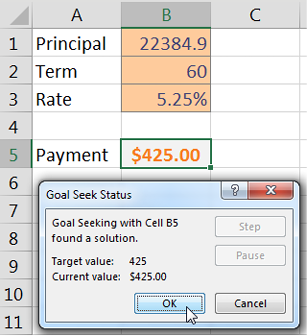
Excel quickly finds that you can get to a $425 car payment if you can get to a $22,384.9 car price.

Note that the formula in B5 stays intact. The only thing that changes is the input value typed in B1.

Also, with Goal Seek, you are free to experiment with changing other input cells. You can still get the $425 loan payment and the $25,995 car if your banker will offer you a 71.3379-month loan!
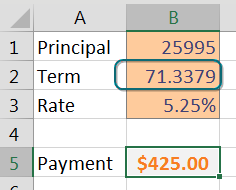
You can Goal Seek based on other cells. Set the Payment to $425 by changing the term and you need a 71.3379 month loan.

Comments

Post a Comment

Popular posts from this blog

Charts - Make your data presentable

One-click charts are easy: Select the data and press  Alt+F1 . What if you would rather create bar charts instead of the default clustered column chart? To make your life easier, you can change the default chart type. Store your favorite chart settings in a template and then teach Excel to produce your favorite chart in response to  Alt+F1 . Say that you want to clean up the chart above. All of those zeros on the left axis take up a lot of space without adding value. Double-click those numbers and change Display Units from None to Millions. To move the legend to the top, click the + sign next to the chart, choose the arrow to the right of Legend, and choose Top. Change the color scheme to something that works with your company colors. Right-click the chart and choose Save As Template. Then, give the template a name. (I called mine ClusteredColumn.) Select a chart. In the Design tab of the Ribbon, choose Change Chart Type. Click on the Templates folder to see the template that ...

Trace Precedents which cells forform into a formula

If you need to see which cells flow into a formula, you can use the Trace Precedents command in the Formula Auditing group on the Formulas tab. In the following figure, select D6. Choose Trace Precedents. Blue lines will draw to each cell referenced by the formula in D6. The dotted line leading to a symbol in B4 means there is at least one precedent on another worksheet. If you double-click the dotted line, Excel shows you a list of the off-sheet precedents. If you stay in cell D6 and choose Trace Precedents a few more times, you will see the second-level precedents, then the third-level precedents, and so on. When you are done, click Remove Arrows.

Vlookup to the Left with Index and Match function

What if your lookup value is to the right of the information that you want VLOOKUP to return? Conventional wisdom says VLOOKUP cannot handle a negative column number in order to go left of the key. One solution is  =VLOOKUP(I7,CHOOSE({1,2},G1:G5,F1:F5),2,0) . However, I prefer to use MATCH to find where the name is located and then use INDEX to return the correct value.