
Goal Seek feature in Excel


Have you ever found yourself plugging in successively higher and lower values into an input cell, hoping to arrive at a certain answer?


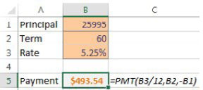
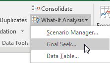
A tool that is built in to Excel does exactly this set of steps. Select the cell with the Payment formula. On the Data tab, in the Data Tools group, look for the What-If Analysis dropdown and choose Goal Seek….

A simple model calculates a loan payment. Choose the payment cell.
Under What-If Analysis, choose Goal Seek.

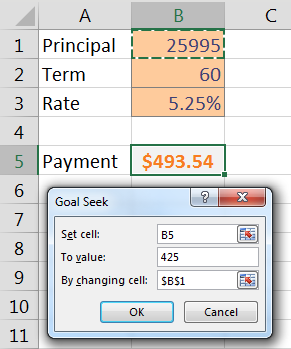
The figure below shows how you can try to set the payment in B5 to $425 by changing cell B1

In the Goal Seek dialog, Set Cell B5 to $425 by changing cell B1.

Goal Seek finds the correct answer within a second.

Excel quickly finds that you can get to a $425 car payment if you can get to a $22,384.9 car price.

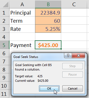
Note that the formula in B5 stays intact. The only thing that changes is the input value typed in B1.

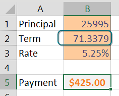
Also, with Goal Seek, you are free to experiment with changing other input cells. You can still get the $425 loan payment and the $25,995 car if your banker will offer you a 71.3379-month loan!

You can Goal Seek based on other cells. Set the Payment to $425 by changing the term and you need a 71.3379 month loan.

Comments

Post a Comment

Popular posts from this blog

Up and Down Markers using Conditional Formatting

There is a super-obscure way to add up/down markers to a pivot table to indicate an increase or a decrease. Somewhere outside the pivot table, add columns to show increases or decreases. In the figure below, the difference between I6 and H6 is 3, but you just want to record this as a positive change. Use  SIGN(I6-H6)  to get either +1, 0, or -1. Select the two-column range showing the sign of the change and then select Home, Conditional Formatting, Icon Sets, 3 Triangles. (I have no idea why Microsoft called this option 3 Triangles, when it is clearly 2 Triangles and a Dash, as shown below.) With the same range selected, now select Home, Conditional Formatting, Manage Rules, Edit Rule. Check the Show Icon Only checkbox. With the same range selected, press  Ctrl+C  to copy. Select the first Tuesday cell in the pivot table. From the Home tab, open the Paste dropdown and choose Linked Picture. Excel pastes a live picture of the icons above the table. At this point, adju...

Indirect Function

INDIRECT  is pretty cool for grabbing a value from a cell. Can  INDIRECT  point to a multi-cell range and be used in a  VLOOKUP  or  SUMIF  function?  You can build an  INDIRECT  function that points to a range. The range might be used as the lookup table in a  VLOOKUP  or as a range in  SUMIF  or  COUNTIF . In  Figure , the formula pulls data from the worksheets specified in row 4. The second argument in the  SUMIF  function looks for records that match a certain date from column A. Note:  Because each worksheet might have a different number of records, I chose to have each range extend to 300. This is a number that is sufficiently larger than the number of transactions on any sheet. The formula in cell B5 is: =SUMIF(INDIRECT(B$4&"!A2:A300"), $A5, INDIRECT(B$4&"!C2:C300")) Summary:  You can use  INDIRECT  to grab data from a multi-cell range.

Create Sum that gives summary of all Worksheets in Excel

  You have a workbook with 12 worksheets, 1 for each month. All of the worksheets have the same number of rows and columns. You want a summary worksheet in order to total January through December. To create it, use the formula  =SUM(January:December!B4) . Copy the formula to all cells and you will have a summary of the other 12 worksheets. Caution I make sure to never put spaces in my worksheet names. If you do use spaces, the formula would have to include apostrophes, like this:  =SUM('Jan 2018:Mar 2018'!B4) .