
Find Largest Value in Excel


MAXIFS

One of the new Office 365 functions added in February 2016 is the MAXIFS function. This function, which is similar to SUMIFS, finds the largest value that meets one or more criteria: You can either hard-code the criterion as in row 7 below or point to cells as in row 9. A similar MINIFS function finds the smallest value that meets one or more criteria.

Amounts appears in D12:D125. To get the Largest, use =MAX($D$12:$D$125). To get the 2nd Largest, use =LARGE($D$12:$D$125,2). To get the 3rd Largest, use =LARGE($D$12:$D$125,3). To get the 3rd Smallest, use =SMALL($D$12:$D$125,3). To get the 2nd Smallest, use =SMALL($D$12:$D$125,2). To get the Smallest, use =MIN($D$12:$D$125). To get the Smallest Widget, use =MINIFS($D$12:$D$125,$B$12:$B$125,"Widget"), To get the Largest with 2 Criteria entered in B8:C8, use =MAXIFS($D$12:$D$125,$B$12:$B$125,B8,$C$12:$C$125,C8)

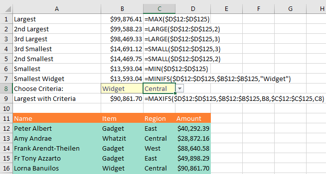
While most people have probably heard of MAX and MIN, but how do you find the second largest value? Use LARGE (rows 2 and 3) or SMALL (rows 4 and 5).

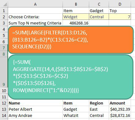
What if you need to sum the top seven values that meet criteria? The orange box below shows how to solve with the new Dynamic Arrays. The green box is the Ctrl+Shift+Enter formula required previously.

Before Dynamic Arrays, you would use: '{=SUM(
AGGREGATE(14,4,($B$13:$B$126=$B$2)
*($C$13:$C$126=$C$2)
*($D$13:$D$126),
ROW(INDIRECT("1:"&D2))))}.
 With Dynamic Arrays, the formula is =SUM(LARGE(FILTER(D13:D126,(B13:B126=B2)*(C13:C126=C21)),SEQUENCE(D2)))

Comments

Popular posts from this blog

40 Power Query Editor features in Power BI

40 Power Query Editor features in Power BI along with examples: 1. Filter Rows: Remove rows based on conditions. Example: Remove rows with a null value in the "CustomerName" column. 2. Remove Duplicates: Eliminate duplicate rows. Example: Remove duplicate entries based on the "OrderID" column. 3. Sort Rows: Arrange rows in ascending or descending order. Example: Sort data by "Date" column in descending order. 4. Replace Values: Substitute one value with another. Example: Replace "N/A" with "Unknown" in the "Status" column. 5. Split Columns: Divide a column into multiple columns. Example: Split "FullName" into "FirstName" and "LastName." 6. Merge Queries: Combine data from multiple sources. Example: Merge customer and order data based on the "CustomerID." 7. Group By: Aggregate data based on a specific column. Example: Group sales data by "ProductCategory" and calculate the sum ...

Recover Unsaved Excel File

We normally avoid these settings but in the hour of need they save us rework time. So if your working on a excel file and you forget to save it or click on don't save by mistake, follow below steps  If the workbook was open for at least 10 minutes and created an AutoRecover version, Excel kept a copy for you. Follow these steps to get it back: Open Excel. In the left panel, choose Open Other Workbooks. In the center panel, scroll all the way to the bottom of the recent files. At the very end, click Recover Unsaved Workbooks. Excel shows you all the unsaved workbooks that it has saved for you recently. Click a workbook and choose Open. If it is the wrong one, go back to File, Open and scroll to the bottom of the list. When you find the right file, click the Save As button to save the workbook. Unsaved workbooks are saved for four days before they are automatically deleted. Use AutoRecover Versions to Recover Files Previously Saved Recover Unsaved Workbooks applies only to files that...

Stockhistory Function

We begin with a list of stock ticker symbols and their respective company names. Our objective is to display the monthly close stock price from a user-defined date to the present.  We also want to display an in-cell line chart that visualizes the monthly price changes while identifying the monthly high and low over the requested time. The  STOCKHISTORY  function retrieves historical data about a financial instrument and loads it as an array, which will spill if it’s the final result of a formula. This means that Excel will dynamically create the appropriately sized array range when you press  ENTER . The syntax for the STOCKHISTORY function is as follows ( optional arguments are in square brackets ): =STOCKHISTORY(stock, start_date, [end_date], [interval], [headers], [property0], [property1], [property2], [property3], [property4], [property5]) stock  – Enter a ticker symbol in double quotes ( g.,  “MSFT” ) or a reference to a cell containing the Stocks data...