Compare two columns with Go To Special

In the figure below, say that you want to find any changes between column A and column D.

There are lists of products in A and D. Select A2:A9. Ctrl+Select D2:D9. Open Home, Find & Select, Go To Special. Choose Row Differences. OK.

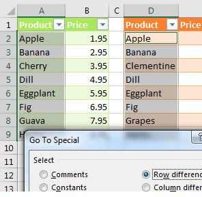
Select the data in A2:A9 and then hold down the Ctrl key while you select the data in D2:D9.

Select, Home, Find & Select, Go To Special. Then, in the Go To Special dialog, choose Row Differences. Click OK.

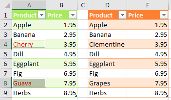
Only the items in column A that do not match the items in column D are selected. Use a red font to mark these items, as shown below.

After choosing Row Differences, any items in column A that do not match column D are highlighted. Apply a red font so you can identify which have changed.

Caution

This technique works only for lists that are mostly identical. If you insert one new row near the top of the second list, causing all future rows to be offset by one row, each of those rows is marked as a row difference

Comments

Data Cleaning Functions in Excel

The CLEAN function Using the CLEAN function removes nonprintable characters text. For example, if the text labels shown in a column are using crazy nonprintable characters that end up showing as solid blocks or goofy symbols, you can use the CLEAN function to clean up this text. The cleaned‐up text can be stored in another column. You can then work with the cleaned text column. The CLEAN function uses the following syntax: CLEAN(text) The text argument is the text string or a reference to the cell holding the text string that you want to clean. For example, to clean the text stored in Cell A1, use the following syntax: CLEAN(A1) The CONCATENATE function The CONCATENATE function combines, or joins, chunks of text into a single text string. The CONCATENATE function uses the following syntax: CONCATENATE(text1,text2,text3,...) The text1, text2, text3, and so on arguments are the chunks of text that you want to combine into a single string. For example, if the city, state, and ZIP co...

Formatting Tips

1. Use tables to format data quickly Excel Tables are an incredibly powerful way to handle a bunch of related data. Just select any cell with in the data and press CTRL+T and then Enter. And bingo, your data looks slick in no time. This has to be the best and easiest formatting tip. 2. Change colors in a snap So you have made a spreadsheet model or dashboard. And you want to change colors to something fresh. Just go to Page Layout ribbon and choose a color scheme from Colors box on top left. Microsoft has defined some great color schemes. These are well contrasted and look great on your screen. You can also define your own color schemes (to match corporate style). What more, you can even define schemes for fonts or combine both and create a new theme. 3. Use cell styles Consistency is an important aspect of formatting. By using cell styles, you can ensure that all similar information in your workbook is formatted in the same way. For example, you can color all input cells in orang...

Rank Function

How to Use the RANK Function If you give the RANK function a number, and a list of numbers, it will tell you the rank of that number in the list, either in ascending or descending order. For example, in the screen shot below, there is a list of 10 student test scores, in cells B2:B11. To find the rank of the the first student's score in cell B2, enter this formula in cell C2: =RANK(B2,$B$2:$B$11) Then, copy the formula from cell C2 down to cell C11, and the scores will be ranked in descending order. RANK Function Arguments There are 3 arguments for the RANK function: number : in the above example, the number to rank is in cell B2 ref : We want to compare the number to the list of numbers in cells $B$2:$B$11 . Use an absolute reference ($B$2:$B11), instead of a relative reference (B2:B11)so the referenced range will stay the same when you copy the formula down to the cells below order : (optional) This argument tells Excel whether to rank the list in ascending or descending o...

Solutions for Data Science

Search This Blog