
3D Map in Excel

3D Maps lets you see five dimensions: latitude, longitude, color, height, and time. Using it is a fascinating way to visualize large data sets.

3D Maps can work with simple one-sheet data sets or with multiple tables added to the Data Model. Select the data. On the Insert tab, choose 3D Map. (The icon is located to the right of the Charts group.) If you have Excel 2013 you might have to download Power Map Preview from Microsoft to use the feature.

3D Map is a new icon to the right of the Charts group on the Insert tab.

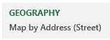
Next, you need to choose which fields are your geography fields. This could be Country, State, County, Zip Code, or even individual street addresses.

You can choose to map by Street Address, Zip Code, State, Country, and so on.

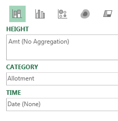
You are given a list of the fields in your data set and drop zones named Height, Category, and Time.

The Height drop zone is sales amount. The Category drop zone contains housing allotment. The Time drop zone contains Sales Date.

Hover over any point on the map to get details such as last sale date and amount.

In the default state of 3D Maps, each data point occupies about one city block. To be able to plot many houses on a street, select the Gear Wheel, Layer Options and change the thickness of the point to 10%.

To get the satellite imagery, open the Themes dropdown and use the second theme.

3D Maps provides a completely new way to look at your data. It is hard to believe that this is Excel.

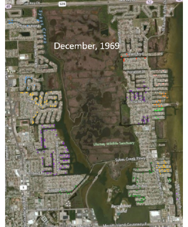
Here is a map of Merritt Island, Florida. The various colors are different housing allotments. Each colored dot on the map is a house with a dock, either on a river or one of many canals dredged out in the 1960s and 1970s.

14 housing allotments are plotted in different colors. In this view from directly overhead, you can't really make out the height of the columns. This view is from March 2013.

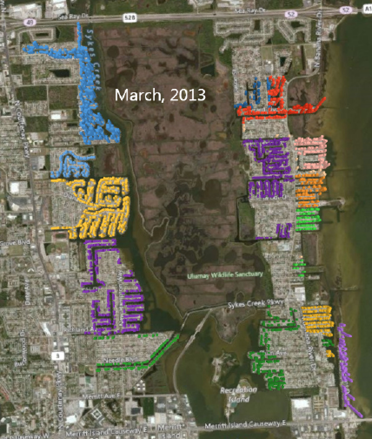
Using the time slider, you can go back in time to any point. Here is the same area at the time when NASA landed the first man on the Moon. The NASA engineers had just started building waterfront homes here, a few miles south of Kennedy Space Center.

Drag the time scrubber back to December 1969 and only 2 of the housing allotments are fully built out. A few scattered houses in newer allotments are just starting to appear.

Use the wheel mouse to scroll in. You can actually see individual streets, canals, and driveways.

Zooming in, you can start to make out individual houses and see some of the sales price height.

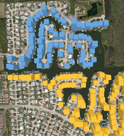
Hold down the Alt key and drag sideways to rotate the map. Hold down the Alt key and drag up to tip the map so your view is closer to the ground.


Comments

Popular posts from this blog

Up and Down Markers using Conditional Formatting

There is a super-obscure way to add up/down markers to a pivot table to indicate an increase or a decrease. Somewhere outside the pivot table, add columns to show increases or decreases. In the figure below, the difference between I6 and H6 is 3, but you just want to record this as a positive change. Use  SIGN(I6-H6)  to get either +1, 0, or -1. Select the two-column range showing the sign of the change and then select Home, Conditional Formatting, Icon Sets, 3 Triangles. (I have no idea why Microsoft called this option 3 Triangles, when it is clearly 2 Triangles and a Dash, as shown below.) With the same range selected, now select Home, Conditional Formatting, Manage Rules, Edit Rule. Check the Show Icon Only checkbox. With the same range selected, press  Ctrl+C  to copy. Select the first Tuesday cell in the pivot table. From the Home tab, open the Paste dropdown and choose Linked Picture. Excel pastes a live picture of the icons above the table. At this point, adju...

Indirect Function

INDIRECT  is pretty cool for grabbing a value from a cell. Can  INDIRECT  point to a multi-cell range and be used in a  VLOOKUP  or  SUMIF  function?  You can build an  INDIRECT  function that points to a range. The range might be used as the lookup table in a  VLOOKUP  or as a range in  SUMIF  or  COUNTIF . In  Figure , the formula pulls data from the worksheets specified in row 4. The second argument in the  SUMIF  function looks for records that match a certain date from column A. Note:  Because each worksheet might have a different number of records, I chose to have each range extend to 300. This is a number that is sufficiently larger than the number of transactions on any sheet. The formula in cell B5 is: =SUMIF(INDIRECT(B$4&"!A2:A300"), $A5, INDIRECT(B$4&"!C2:C300")) Summary:  You can use  INDIRECT  to grab data from a multi-cell range.

Create Sum that gives summary of all Worksheets in Excel

  You have a workbook with 12 worksheets, 1 for each month. All of the worksheets have the same number of rows and columns. You want a summary worksheet in order to total January through December. To create it, use the formula  =SUM(January:December!B4) . Copy the formula to all cells and you will have a summary of the other 12 worksheets. Caution I make sure to never put spaces in my worksheet names. If you do use spaces, the formula would have to include apostrophes, like this:  =SUM('Jan 2018:Mar 2018'!B4) .