Change from Lower to Upper Case in Excel

1. Insert a new blank column to the right of your data.
2. Use a formula such as =UPPER(D2). To convert to lower case, use =LOWER(). To convert to Proper case, use =PROPER().
3. Copy the temporary formula down to all rows by double-clicking the fill handle.
4. The entire range of new formulas will be selected. Press Ctrl+C to copy.
5. Press the left arrow to move to the original data. Right-click and choose Paste Values.

6. You can now delete the temporary column D.

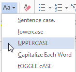
Additional Details: I to bring up the “W” program again, but here is another place where Microsoft Word could make this easier. If you had an entire table that needs converting, select the whole table, paste to a blank word document, then use the Change Case dropdown in the Home tab.

After the conversion is done, copy from Word and paste back to Excel.

Microsoft Word offers a Aa drop-down menu with Sentence Case, lowercase, UPPERCASE, Capitalize Each Word and tOGGLE cASE

#upper #Uppercase

Comments

Rank Function

How to Use the RANK Function If you give the RANK function a number, and a list of numbers, it will tell you the rank of that number in the list, either in ascending or descending order. For example, in the screen shot below, there is a list of 10 student test scores, in cells B2:B11. To find the rank of the the first student's score in cell B2, enter this formula in cell C2: =RANK(B2,$B$2:$B$11) Then, copy the formula from cell C2 down to cell C11, and the scores will be ranked in descending order. RANK Function Arguments There are 3 arguments for the RANK function: number : in the above example, the number to rank is in cell B2 ref : We want to compare the number to the list of numbers in cells $B$2:$B$11 . Use an absolute reference ($B$2:$B11), instead of a relative reference (B2:B11)so the referenced range will stay the same when you copy the formula down to the cells below order : (optional) This argument tells Excel whether to rank the list in ascending or descending o...

Formatting Tips

1. Use tables to format data quickly Excel Tables are an incredibly powerful way to handle a bunch of related data. Just select any cell with in the data and press CTRL+T and then Enter. And bingo, your data looks slick in no time. This has to be the best and easiest formatting tip. 2. Change colors in a snap So you have made a spreadsheet model or dashboard. And you want to change colors to something fresh. Just go to Page Layout ribbon and choose a color scheme from Colors box on top left. Microsoft has defined some great color schemes. These are well contrasted and look great on your screen. You can also define your own color schemes (to match corporate style). What more, you can even define schemes for fonts or combine both and create a new theme. 3. Use cell styles Consistency is an important aspect of formatting. By using cell styles, you can ensure that all similar information in your workbook is formatted in the same way. For example, you can color all input cells in orang...

Turn Data Sideways

Someone built this lookup table sideways, stretching across C1:N2. I realize that I could use HLOOKUP instead of VLOOKUP, but I prefer to turn the data back to a vertical orientation. Copy C1:N2. Right-click in A4 and choose the Transpose option under the Paste Options. Transpose is the fancy Excel word for “turn the data sideways.” I transpose a lot. But I use Alt+E , S , E , Enter to transpose instead of the right-click. There is a problem, though. Transpose is a one-time snapshot of the data. What if you have formulas in the horizontal data? Is there a way to transpose with a formula? The first way is a bit bizarre. If you are trying to transpose 12 horizontal cells, you need to select 12 vertical cells in a single selection. Start typing a formula such as =TRANSPOSE(C2:N2) in the active cell but do not press Enter. Instead, hold down Ctrl+Shift and then press Enter . This puts a single array formula in the selected cells. T...

Solutions for Data Science

Search This Blog